How to expand a table's width over the page margins?

I have a margin on the page set to something like - (left: 4cm, bottom: 2cm, top: 2cm, right: 2cm)

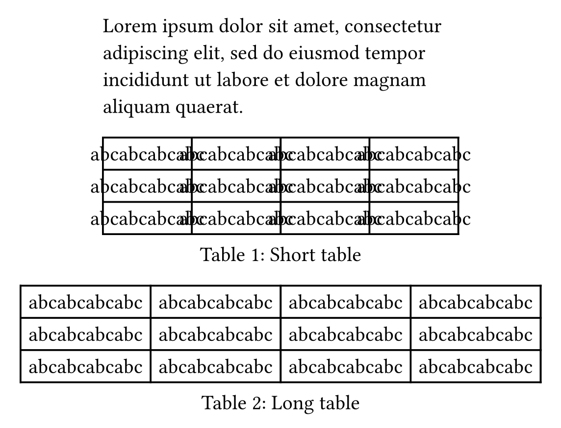
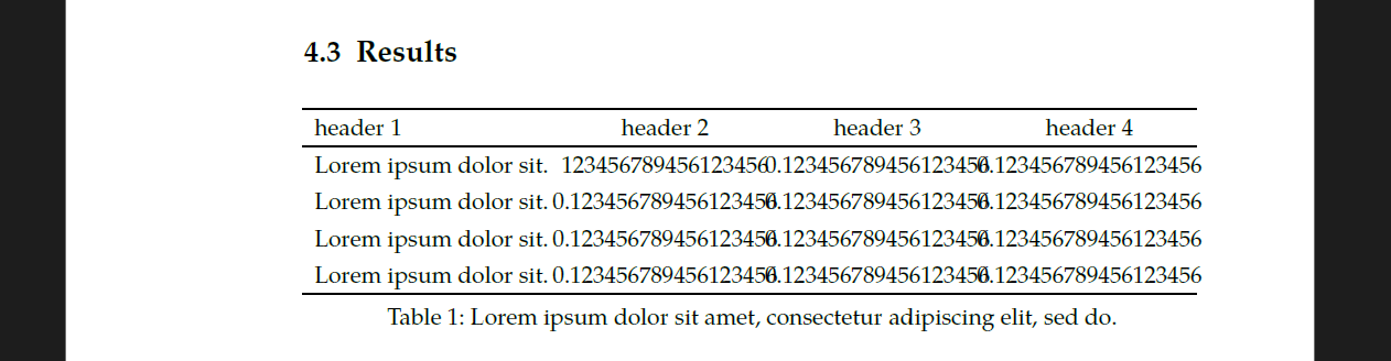
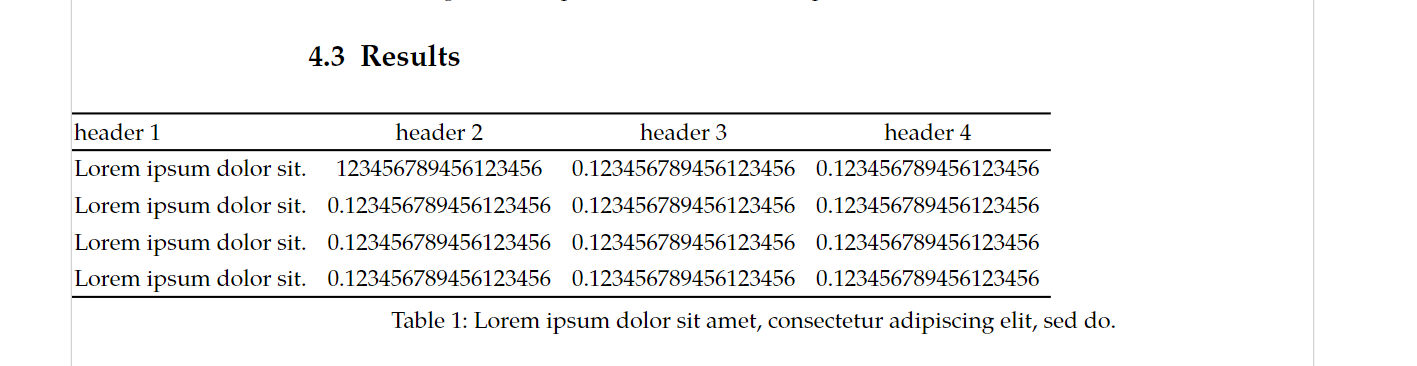
How should I increase the width of the table? It looks like this

and here is my code

#figure(
  box(width: 15fr, table(
    stroke: none,
    columns: (auto, 2fr, 2fr, 2fr),
    align: (left, center, center, center),
    table.hline(),
    table.header(
      [header 1], [header 2], [header 3], [header 4],
    ),
    table.hline(),
    [#lorem(4)],[123456789456123456],[0.123456789456123456], [0.123456789456123456],
    [#lorem(4)], [0.123456789456123456], [0.123456789456123456], [0.123456789456123456],
    [#lorem(4)], [0.123456789456123456], [0.123456789456123456], [0.123456789456123456],
    [#lorem(4)], [0.123456789456123456], [0.123456789456123456], [0.123456789456123456],
    table.hline(),
  )),
  caption: [#lorem(10)],
)

I tried adding the box but that does nothing

Update

I tried block instead of box and set it’s width, but it expands only to the left and not to the center or right

Code
#figure(
  block(width: 60em, table(
    stroke: none,
    columns: (auto,) + 3 * (auto,),
    align: (left, center, center, center),
    table.hline(),
    table.header(
      [header 1], [header 2], [header 3], [header 4],
    ),
    table.hline(),
    [#lorem(4)],[123456789456123456],[0.123456789456123456], [0.123456789456123456],
    [#lorem(4)], [0.123456789456123456], [0.123456789456123456], [0.123456789456123456],
    [#lorem(4)], [0.123456789456123456], [0.123456789456123456], [0.123456789456123456],
    [#lorem(4)], [0.123456789456123456], [0.123456789456123456], [0.123456789456123456],
    table.hline(),
  )),
  caption: [#lorem(10)],
)

Wrapping the table in a call to align achieves this:

#figure(
  block(width: 60em,
    align(center, //Align starts here
      table(
        stroke: none,
        columns: (auto,) + 3 * (auto,),
        align: (left, center, center, center),
        table.hline(),
        table.header(
          [header 1], [header 2], [header 3], [header 4],
        ),
        table.hline(),
        [#lorem(4)],[123456789456123456],[0.123456789456123456], [0.123456789456123456],
        [#lorem(4)], [0.123456789456123456], [0.123456789456123456], [0.123456789456123456],
        [#lorem(4)], [0.123456789456123456], [0.123456789456123456], [0.123456789456123456],
        [#lorem(4)], [0.123456789456123456], [0.123456789456123456], [0.123456789456123456],
        table.hline(),
      )
    ) //Align ends here
  ),
  caption: [#lorem(10)],
)
1 Like

You can use pad with negative lengths to “bypass” the margins:

#set page(margin: (x: 5em))

#lorem(20)

#figure(table(
  columns: (1fr,) * 4,
  ..([abcabcabcabc],)*4*3
), caption: [Short table])

#pad(x: -4em, figure(table(
  columns: (1fr,) * 4,
  ..([abcabcabcabc],)*4*3
), caption: [Long table]))

By the way, I’ve updated your post title to better fit our guidelines: How to post in the Questions category

Please ensure your title is a Typst question you’d ask to a friend. :slight_smile:

1 Like

I tried doing this, but using pad worked. Thanks for the help

Is there a nicer way to do this besides using manual padding? @gezepi 's solution looks clean, but it doesn’t work for me:

  #figure(
      align(center,
          table(
              table.header([Symbol], [Meaning], [Description], [Shape]),
              align: horizon,
              columns: (5em, 10em, 14em, 12em),
              $f$, [Forward operator], [Mapping from 3D H-density to column density], [$f: bb(R)^3 → bb(R)^3$ (static) \ $f: bb(R)^4→bb(R)^3$ (dynamic)],
              $m$, [Model], [Mapping from model parameters to 3D H-density], [$m: bb(R)^* → bb(R)^3$ (static) \ $m: bb(R)^* → bb(R)^4$ (dynamic)],
              $bold(c)$, [Model params.], "Free model variables,\n usually low-dimensional.", [$bold(c) ∈ bb(R)^*$ \ \* model dependent],
              $bold(y)$, [Measurements.], "Column densities measured\n by instrument", [$bold(y) ∈ bb(R)^3$],
          ),
      ),
      caption: [Symbols],
      // FIXME: move to glossary section?
  )

  An inverse problem is the procedure of determining the causative factors of a set of measurements derived from some observation process.  In exospheric tomography, the factor driving the intensity of column density measurements is the distribution of hydrogen in the regions being observed.  In general, a direct analytic solution to tomography or other inverse problems is not feasible, so numerical approximations and discretization become necessary.  In this chapter, I lay out key concepts of linear inverse problems, detail discretization for approaching tomographic inversion numerically, and introduce notation which will be used later in the manuscript to describe tomographic retrieval algorithms.

Hello @Evon_Vootlo
have you tried this?

I have, but I want to avoid manual padding because it has to been changed if the table width changes.

Ah indeed! I didn’t understand that, sorry.
you can just use a show rule and pad by 50%

#show figure: f => {
  pad(x: -50%, f)
}

Thanks for the tip! Here’s the inline version for posterity:

 #figure(
      pad(x: -50%,
          table(
              table.header([Symbol], [Meaning], [Description], [Shape]),
              align: horizon,
              columns: (5em, 10em, 14em, 12em),
              $f$, [Forward operator], [Mapping from 3D H-density to column density], [$f: bb(R)^3 → bb(R)^3$ (static) \ $f: bb(R)^4→bb(R)^3$ (dynamic)],
              $m$, [Model], [Mapping from model parameters to 3D H-density], [$m: bb(R)^* → bb(R)^3$ (static) \ $m: bb(R)^* → bb(R)^4$ (dynamic)],
              $bold(c)$, [Model params.], "Free model variables,\n usually low-dimensional.", [$bold(c) ∈ bb(R)^*$ \ \* model dependent],
              $bold(y)$, [Measurements.], "Column densities measured\n by instrument", [$bold(y) ∈ bb(R)^3$],
          ),
      ),
      caption: [Symbols],
      // FIXME: move to glossary section?
  )

  An inverse problem is the procedure of determining the causative factors of a set of measurements derived from some observation process.  In exospheric tomography, the factor driving the intensity of column density measurements is the distribution of hydrogen in the regions being observed.  In general, a direct analytic solution to tomography or other inverse problems is not feasible, so numerical approximations and discretization become necessary.  In this chapter, I lay out key concepts of linear inverse problems, detail discretization for approaching tomographic inversion numerically, and introduce notation which will be used later in the manuscript to describe tomographic retrieval algorithms.

1 Like